前回で最適化計算が終了したので、今回はこれら計算結果の表示・評価について紹介する。
表示項目については、例題マニュアル P14 Exercises からいくつかの項目を抜き出して紹介する。
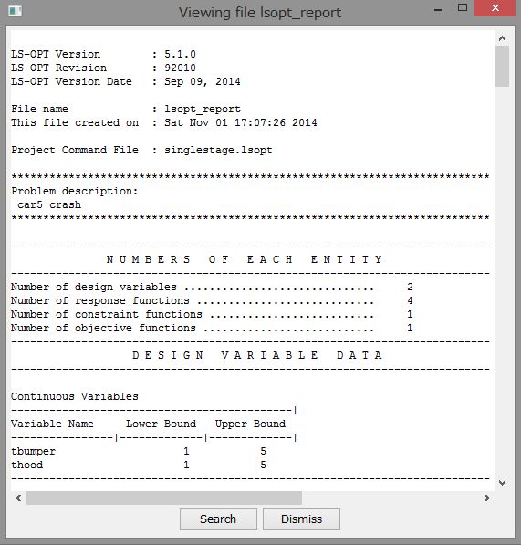
初めに、P16 File Viewingから。マニュアルでは最後の手順になっているが、設定通り計算できたかどうか、初めにこの表示で確認するべきである。
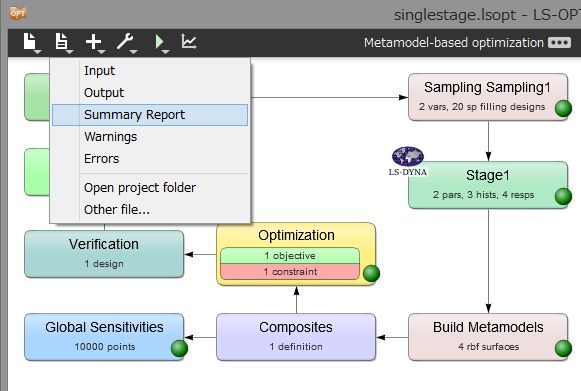
lsoptui – File Menu – Summary Report
計算結果は、作業フォルダ- Stage1(ユーザ設定) – 収束回数.サンプリング回数 フォルダに格納される。
今回の例では、C:\temp^lsopt1\Stage1\1.1 – 1.20 & 2.1 フォルダの下に計算結果ファイルが存在している。
設定が間違っていなければ、以下のようなサマリーが表示されるはずだ。
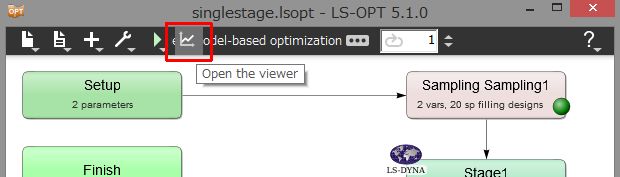
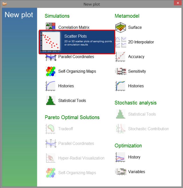
描画メニューの起動
以下、例題マニュアルの順に紹介していく。
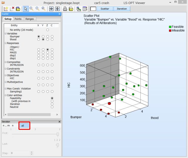
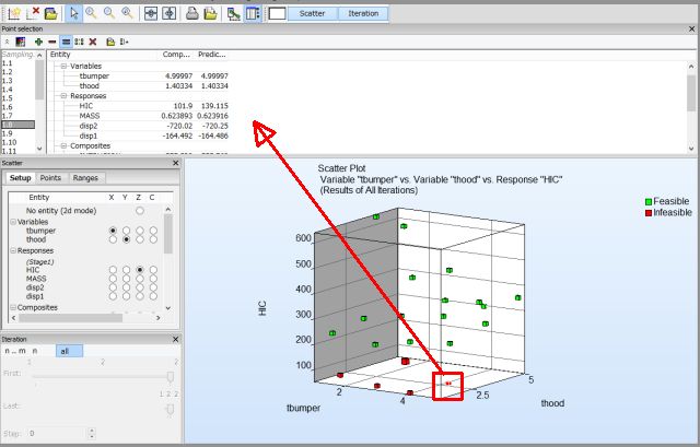
1.Scatter Plot
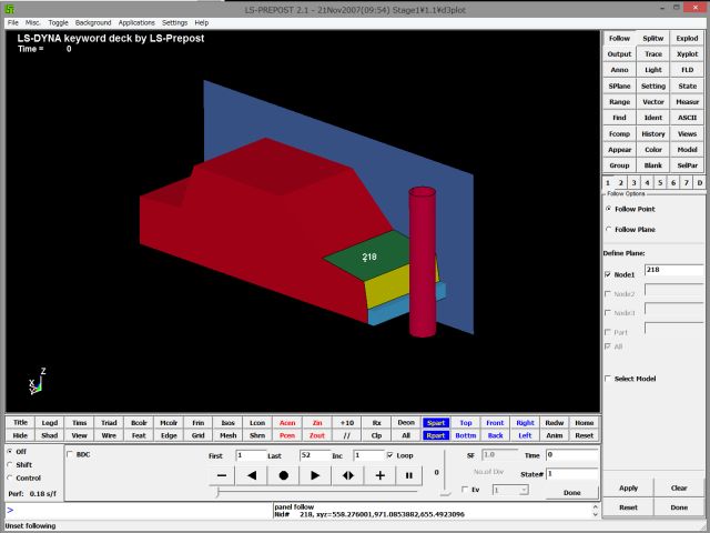
1.1 Find the Baseline design ( Design 1.1 ) and display the FEM using LSPP
Itaration all を選択 (以降の操作に共通)
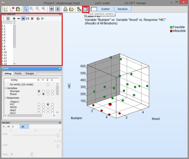
1.1を選択して、LSPPアイコンを選択
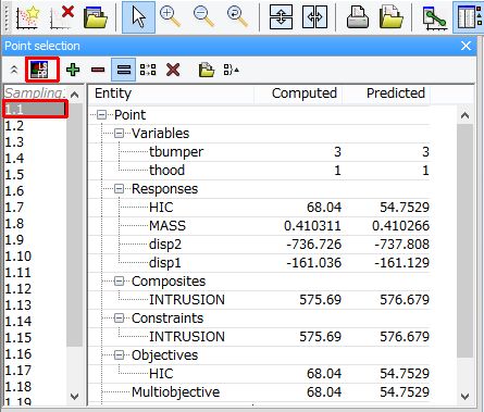
LSPP (Ver2.1)が起動、モデルが表示される。LSPPはかなり古いバージョンで現在とはメニュースタイルが異なる。
1.3 Select the Infeasible Points – 赤のポイントを選択
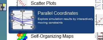
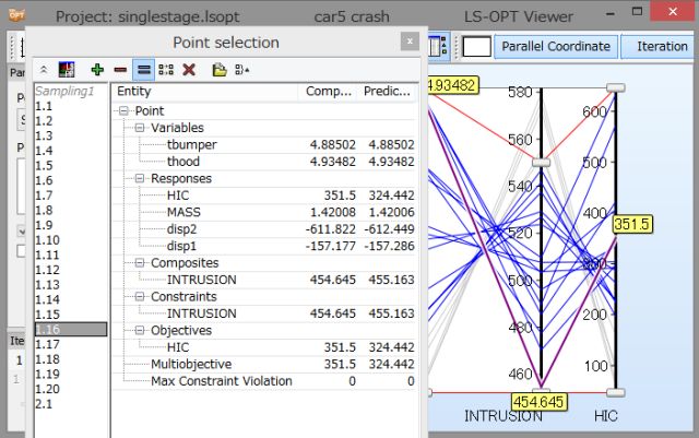
2. Parallel Coordinate Plot
2.1 Display the Variables, Constraints, Objectives
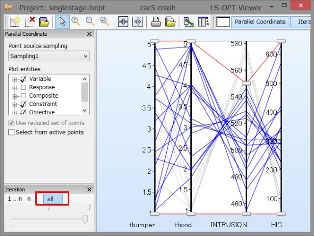
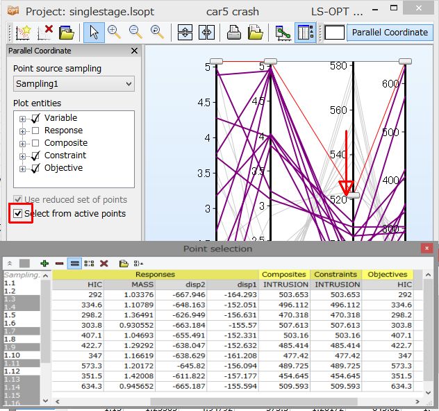
2.3 Find a feasible point with the lowest Intrusion
2.4 Slide the upper bound of the Intrusion to 520 : 条件を満たすデザインのみが選択される。
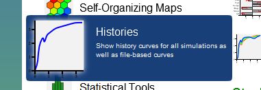
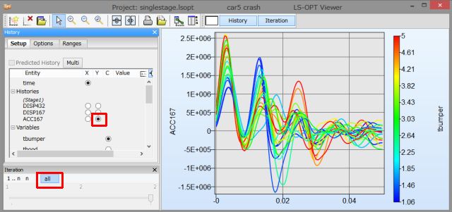
3.Histories
3.1 Display All the ACCE histories
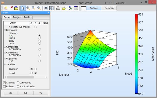
3.Metamodel Surface
3.1 Display the Metamodel Surface for the HIC function.
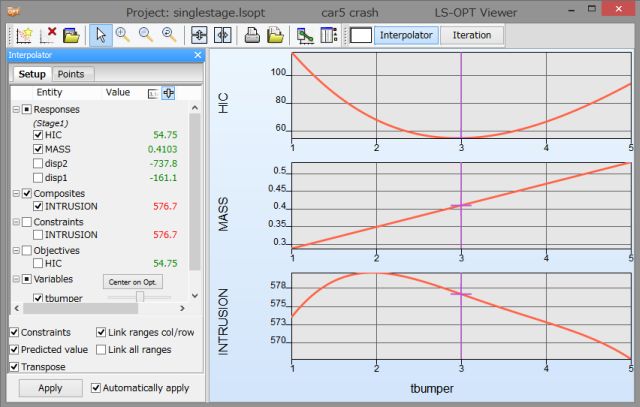
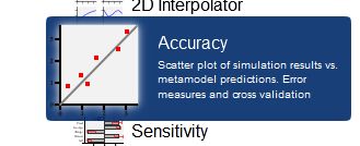
5.2D Interpolator
5.1 & 5.2 – Select Constraints, Predicted Value, Transpose and Link Ranges
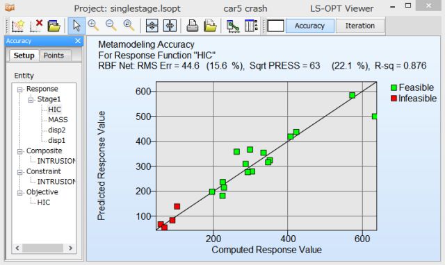
6.Metamodel Accuracy
6.1 Study and compare the PRESS value for HIC, Mass,,,,,
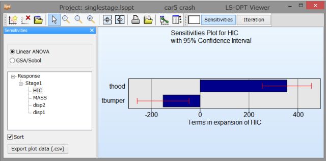
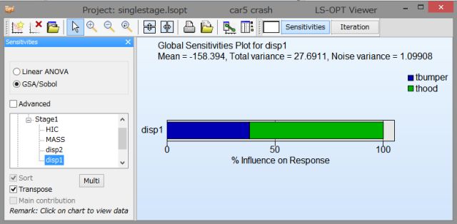
7.Sensitivities
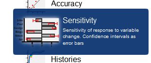
7.1 Using Linear ANNOVA
7.3 In the GSA/Sobol, 7.4 Display the Transpose
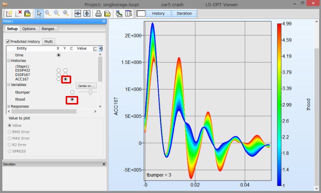
8.Predicted Histories
8.1 Select the ACCE
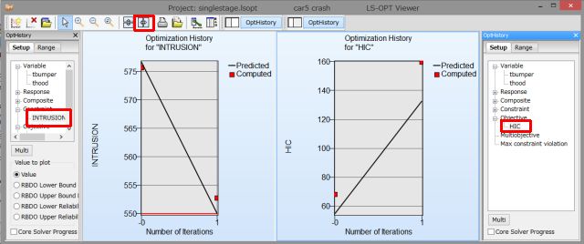
9. Optimization History
9.1 View the HIC and Intrusin by selecting “Split”